

Volatility-adjusted returns measure how much profit you earn for the risk you take. The goal? Smarter trading decisions that balance returns with risk. Here's what matters most:
- Key Metrics: Use the Sharpe ratio (total risk) and Sortino ratio (downside risk) to evaluate performance. A Sharpe ratio above 1.0 is solid; over 3.0 might signal issues.
- Volatility Targeting: Adjust your portfolio exposure based on market volatility. For example, reduce positions during high-volatility periods (e.g., VIX > 25) to limit losses.
- Position Sizing: Size trades based on volatility, often using the Average True Range (ATR). This ensures consistent risk across assets.
- Correlation: Diversify effectively by monitoring correlations. Assets with high correlation (>0.6) amplify risk, so adjust position sizes accordingly.
- Stress Testing: Simulate extreme scenarios (like 2008 or 2020 crashes) to ensure your strategy can handle market shocks.
Smart risk management, not just chasing returns, separates professional traders from gamblers. By focusing on volatility, correlation, and proper sizing, you can improve your trading outcomes over time.
Volatility-Adjusted Sizing vs Equal Weighting | Which Wins?
Position Sizing and Volatility Targeting
Traders often obsess over finding the perfect entry signals, but studies show that position sizing plays a much bigger role - accounting for about 90% of the variation in trading outcomes when comparing identical entry signals with different sizing methods. In short, getting the size right is far more impactful than many realize, which is why you should manage risk like a professional.
Volatility Targeting at the Portfolio Level
One effective strategy for managing portfolio risk is to scale your total exposure based on recent market volatility. The idea is simple: increase exposure during calm periods and reduce it when volatility spikes. This works because volatility tends to be predictable. For example, a 21-day realized variance estimate has a strong autocorrelation of 0.7–0.8, meaning periods of high or low volatility often persist. By adjusting exposure early, you can avoid reacting too late after losses have already piled up.
Here’s a concrete example: during the 2008 Global Financial Crisis, a volatility-targeted strategy cut the S&P 500 drawdown from –37.0% to –21.4%. Similarly, during the 2020 COVID crash, it reduced the peak-to-trough drawdown by roughly 15 percentage points.
A practical way to implement this is by using a VIX-based regime table:
| VIX Regime | Volatility State | Position-Size Scalar | Action |
|---|---|---|---|
| Regime 1 (<16) | Low | 1.0x | Maintain full baseline size |
| Regime 2 (16–25) | Elevated | 0.6x – 0.75x | Scale down; expect more choppiness |
| Regime 3 (>25) | High | 0.3x – 0.5x | Significantly reduce exposure; high gap risk |
To avoid extremes, two safeguards are essential:
- Leverage Cap: Limit leverage to 1.5x–2.0x during calm periods to prevent overexposure.
- Volatility Floor: Set a floor (around 6%–8%) to avoid taking oversized positions when volatility drops too low.
Volatility-Based Position Sizing Per Trade
At the trade level, position sizing should also reflect the specific volatility of each asset. It doesn’t make sense to allocate the same dollar amount to a high-volatility asset as you would to a low-volatility one. Instead, trades should be sized to equalize dollar risk across the board.
The formula for this is straightforward:
Position Size = Dollar Risk per Trade ÷ (ATR Multiplier × ATR × Point Value)
.
Interestingly, 68% of professional traders rely on Average True Range (ATR) for sizing their trades. Backtests have shown that ATR-based sizing can improve the Sharpe ratio of a momentum strategy by 34% compared to equal-dollar sizing over a 20-year period.
"Position sizing based on volatility (ATR) is the single most important factor in determining trading system performance, more important than entry signals." - Van Tharp, Trading Psychologist
Here’s a quick guide for ATR multipliers:
- 1.5x ATR: Best for momentum trades.
- 2x ATR: Suitable for standard swing trades.
- 3x ATR: Ideal for longer-term positions.
Always round down the final position size to the nearest lot or share. Rounding up might seem small, but across hundreds of trades, it can lead to unintended risk accumulation.
Finally, to protect against extended losing streaks, apply drawdown limits:
- If your account drops 5% from its peak, reduce risk per trade by 25%.
- For a 10%–15% drop, cut risk by 50% and focus only on your highest-confidence setups.
This approach ensures that a tough stretch doesn’t spiral into a major setback.
Building Portfolios Around Correlation
Once position sizing is in place, the next step is understanding how assets interact - this is where correlation comes into play. Correlation plays a big role in determining overall portfolio risk. By combining correlation insights with volatility-based sizing, you create a more complete framework for managing risk.
Building Low-Correlation Portfolios
As Harry Markowitz, a Nobel laureate, famously said:
"Diversification is the only free lunch in investing."
When assets don't move together in perfect sync, the portfolio's overall risk (or variance) can be lower than the weighted average of individual asset risks. For example, in a portfolio of 30 randomly chosen stocks, roughly 90% of asset-specific risk (also called idiosyncratic risk) can be reduced.
However, diversification works only if the assets behave differently under various conditions. As MQL5 Articles points out:
"A portfolio of five gold scalpers is not diversification - it is concentration disguised as variety."
True diversification means including assets that thrive in different economic environments. For instance, commodities often perform well during stagflation, a period when both stocks and bonds tend to struggle. A clear example of this was during the inflation shock of 2022. A diversified five-asset portfolio (40% stocks, 25% bonds, 15% commodities, 15% real estate, 5% gold) lost just 9.25%, compared to a traditional 60/40 portfolio, which dropped 16%. The commodities portion of the diversified portfolio gained 16%, helping to offset losses.
To avoid unexpected convergence of assets, it’s better to rely on rolling 60-day or 1-year correlation windows rather than static historical averages. Correlations between assets change over time. For example, stocks and bonds were positively correlated from the mid-1960s to the late 20th century. This would have made the assumptions behind today’s 60/40 portfolios unreliable during that period.
Correlation-Adjusted Position Sizing
After building a low-correlation portfolio, it’s important to adjust position sizes using risk calculators and sizing tools based on how much assets are linked to one another. Simply knowing two assets are correlated isn’t enough - you need to act on that information. Correlation can amplify risk in ways that aren’t immediately obvious. For example, three trades with a 90% correlation behave almost like a single trade with triple the risk.
A straightforward system for handling this is:
| Correlation Range (|r|) | Assessment | Action |
|---|---|---|
| < 0.35 | Excellent | Positions are largely independent; no changes needed. |
| 0.35 – 0.60 | Acceptable | Moderate overlap; consider slight size reductions. |
| ≥ 0.60 | Dangerous | High overlap; reduce size significantly or treat as a single position. |
This system provides a clear guideline for adjusting exposure when dealing with highly correlated assets. For example, if you add a position that has a high correlation with your existing holdings, reduce the combined allocation by 30–50%. To better estimate your portfolio's true risk, you can use this formula:
Effective Risk = Nominal Risk × √(N × Average Correlation)
Here’s how it works: If a trader holds five positions, each with 1% nominal risk, and the average pairwise correlation is 0.80, the effective risk isn’t 5%. It’s closer to 10%.
The key takeaway is to focus on how much risk each asset contributes, not just how much capital you’ve allocated. For instance, in a traditional 60/40 portfolio, nearly 90% of the portfolio’s risk comes from stocks because of their higher volatility. A better approach is to size positions so that all assets contribute equally to the portfolio’s overall volatility - this is known as a risk parity strategy. It’s a more balanced way to build a diversified portfolio.
Applying These Strategies in Simulated Trading
Understanding position sizing and correlation management is one thing - putting these principles into practice under market conditions is another. Simulated trading provides a risk-free way to refine your approach before committing real funds.
Testing Volatility Targeting in Demo Accounts
Volatility targeting begins with adjusting position sizes based on current market conditions. A common formula used is:
Position Size = (Risk % × Portfolio Size) / ATR
This ensures consistent risk allocation across different instruments, accounting for market volatility.
Demo accounts are particularly useful for testing this approach because they highlight the limitations of static position sizing. As Algomatic Trading explains:
"Static position sizing isn't just ineffective, it's dangerous. And if you're using it in your backtests, you're not testing what you think you're testing." – Algomatic Trading
To validate your volatility-targeting rules, consider running Monte Carlo simulations. These generate thousands of synthetic equity curves, offering insights into potential outcomes. For example, one GARCH-based volatility timing strategy achieved a median Sharpe ratio of 0.87, with an 82.3% chance of exceeding a Sharpe of 0.5 across 1,000 simulated return paths. It's generally recommended to demo trade strategies for at least three months across various market conditions before moving to live trading.
Once you've built confidence in volatility targeting, the next step is to examine how asset relationships influence overall portfolio risk.
Using Correlation Analysis in Simulated Portfolios
Correlation analysis in simulated portfolios helps uncover hidden concentration risks, allowing you to optimize risk-adjusted returns. A rolling correlation matrix is a handy tool for this, offering a heat map of pairwise correlations among your holdings. The rolling window length should align with your trading style:
- 10–20 days for day trading
- 30–60 days for swing trading
- 90–252 days for position trading
This method becomes especially valuable during periods of market stress. Testing your portfolio against historical crises - like 2008, 2020, or 2022 - can reveal how positions behave when correlations spike toward 1.0.
In simulations, aim to cap effective exposure to any single risk factor at 2–3%, and flag asset pairs with correlations above 0.7 for position size adjustments. This practice can help avoid the kind of concentration risks that contributed to 68% of hedge fund failures between 2000 and 2020.
Using For Traders to Develop Risk-Adjusted Strategies

Once you've validated your strategies in simulations, platforms like For Traders allow you to test them in real-time, controlled environments. The platform’s AI-driven risk management tools and real-time drawdown monitoring make it easier to refine volatility- and correlation-aware strategies without the emotional pressure of live trading.
One standout feature is automated drawdown protection. This tool monitors unrealized P&L in real time and automatically closes all open positions if losses hit a predefined threshold. This acts as a circuit breaker, keeping simulated losses manageable and providing a safety net for aggressive strategies.
Monitoring and Improving Risk-Adjusted Performance
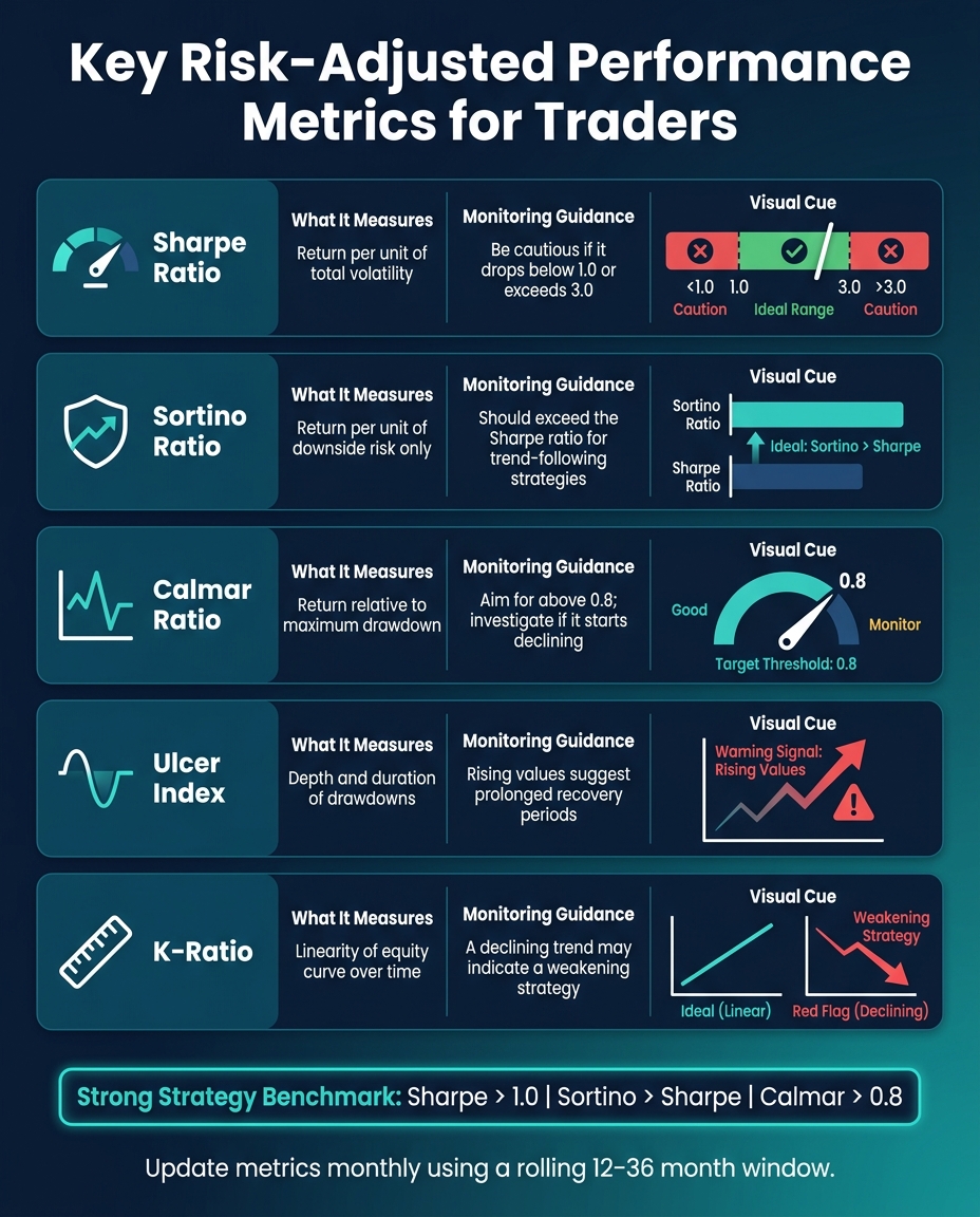
Key Risk-Adjusted Performance Metrics for Traders
Once your volatility-targeting and correlation strategies are in motion, the ongoing task is evaluating whether your risk-adjusted returns are actually improving over time.
Key Risk-Adjusted Metrics to Track
To effectively monitor performance, you’ll need to track multiple metrics, each highlighting a different aspect of risk-adjusted returns.
The Sharpe ratio is widely used in the industry, measuring excess return relative to total volatility. A Sharpe ratio above 1.0 is often considered solid, but anything over 3.0 might indicate data smoothing or manipulation. The Sortino ratio works well for trend-following strategies since it focuses only on downside volatility, ignoring the profitable upside. For those sensitive to drawdowns, the Calmar ratio offers a reality check by comparing annualized returns to the worst peak-to-trough loss.
Ideally, a strong strategy will show a Sharpe above 1.0, a Sortino ratio higher than the Sharpe, and a Calmar above 0.8. Updating these metrics monthly with a rolling 12–36-month window can help identify performance issues before they escalate.
| Metric | What It Measures | Monitoring Guidance |
|---|---|---|
| Sharpe Ratio | Return per unit of total volatility | Be cautious if it drops below 1.0 or exceeds 3.0 |
| Sortino Ratio | Return per unit of downside risk | Should exceed the Sharpe ratio for trend-following |
| Calmar Ratio | Return relative to max drawdown | Aim for above 0.8; investigate if it starts declining |
| Ulcer Index | Depth and duration of drawdowns | Rising values suggest prolonged recovery periods |
| K-Ratio | Linearity of equity curve over time | A declining trend may indicate a weakening strategy |
Using these metrics, you can adjust your portfolio as market conditions evolve.
Rebalancing Based on Volatility and Correlation Changes
Rebalancing takes into account the realities of volatility clustering and shifting correlation dynamics. Volatility often appears in clusters - high-volatility periods tend to follow each other. This makes it possible to predict when position sizes need to be reduced. The formula for scaling exposure is simple: Weight = Target Volatility / Realized Volatility, often calculated using a 21-day trailing window.
Rather than sticking to a fixed schedule, consider rebalancing bands - adjust positions only when they deviate significantly from the target weight. This approach minimizes transaction costs while maintaining risk control. Weekly rebalancing strikes a balance between responsiveness and avoiding excessive trading. During market stress, such as the March 2020 COVID crash, pay close attention to pairwise correlations. For example, during that period, S&P 500 stock correlations spiked from 0.30 to 0.85, effectively reducing the benefits of diversification.
In addition to periodic rebalancing, stress testing helps ensure your strategy can withstand extreme market conditions.
Stress Testing and Scenario Analysis
Standard metrics often assume normal returns, which can overlook extreme, fat-tailed events. Stress testing fills this gap.
Use historical scenarios, such as the 2008 financial crisis or the March 2020 market crash, combined with synthetic shocks that test unlikely but plausible combinations - like a 35% equity drop paired with a 300-basis-point rate increase. For instance, one simulation with such a synthetic shock revealed an average peak-to-trough loss of -39.1% and a median recovery time of 4.3 years. Monte Carlo simulations add another layer by generating thousands of alternative return paths, offering better estimates of tail risk. For reliable 99th-percentile results, aim for 50,000 to 200,000 simulated paths.
"Your backtest's max drawdown is a sample of one. Monte Carlo turns that one into a thousand and asks you to plan against the worst-case you can stomach, not the average." – Quant Trading Tools
To test robustness, tweak parameters by ±5% to ±25% and re-run the strategy. If minor changes cause the strategy to fail, it may have been overfitted to historical noise or influenced by bias in backtesting rather than built on a solid foundation. Together, these steps - monitoring, rebalancing, and stress testing - are essential for maintaining strong risk-adjusted performance.
Conclusion: Key Takeaways for Volatility-Adjusted Returns
Improving risk-adjusted returns isn’t about perfecting your entry points - it’s about how you manage risk at every step. As TradeAlgo puts it:
"Position sizing determines survival, not entries."
The strategies discussed here all revolve around one central principle: prioritize managing your risk, and the returns will follow.
The numbers speak for themselves. Adding a volatility-targeting overlay to the U.S. equity market has been shown to boost the Sharpe ratio by 20% to 40%. Meanwhile, traders who use systematic position sizing have a 47% higher survival rate over three years compared to those who rely on intuition. This can be the difference between thriving in the market and draining your capital.
Here are some key points to keep in mind for effective risk management:
- Adjust exposure based on volatility: Use a 21-day trailing window to scale your exposure inversely to realized volatility.
- Set clear portfolio limits: Keep your total exposure within a range of 5% to 15%, depending on your personal risk tolerance.
- Watch rolling correlations: Static correlations can be misleading. Be prepared to reduce risk quickly when correlations spike, as they did during the March 2020 market turmoil.
- Re-risk cautiously: Volatility shocks often come in waves, so it’s safer to increase exposure more gradually than you reduce it.
- Track performance metrics: Declining metrics are often a red flag that your risk management approach needs adjustment.
These disciplined, systematic methods are the foundation of long-term trading success.
If you’re looking to build these skills in a safe environment, platforms like For Traders offer simulated trading challenges. These allow you to practice strategies like volatility targeting and correlation-aware position sizing without risking real money. This kind of preparation can help you develop the discipline needed to tackle real-world market conditions confidently.
FAQs
How do I choose a realistic target volatility for my portfolio?
To begin, assess your risk tolerance alongside the average long-term volatility of your investments. For context, institutional portfolios often aim for an annualized volatility of 5%-10%, whereas trend-following strategies might target a range of 10%-20%. U.S. equities generally average around 15%-16%.
If you set higher volatility targets, your exposure to risk increases, while lower targets result in a more conservative portfolio. To keep risk in check, especially during periods of low realized volatility, consider implementing leverage caps. This approach helps maintain balance and prevents excessive risk-taking.
What’s the simplest way to volatility-size a trade with ATR in practice?
To adjust your trade size based on market volatility using the Average True Range (ATR), you can align your stop-loss to account for market fluctuations and maintain consistent dollar risk. Here's how:
- Determine your dollar risk per trade: For instance, set it as 1% of your total account equity.
- Calculate the stop-loss distance: Use the formula
ATR × Multiplier(e.g., 2x ATR). - Calculate your position size: Divide your dollar risk by the stop-loss distance (
Dollar Risk ÷ Stop Distance).
This approach ensures your position size adapts to volatility, keeping your risk exposure steady.
How can I reduce risk when my positions become highly correlated?
When managing highly correlated positions, it’s wise to treat them as a single directional bet. If a new trade has a correlation coefficient above 0.7 with your existing positions, you should adjust the combined exposure to ensure it stays within your risk limits. One effective approach is to scale your position sizes inversely to the level of correlation - the higher the correlation, the smaller the position size.
For Traders offers advanced tools that can help you track and manage this type of exposure, ensuring your capital remains protected while maintaining disciplined trading practices.
Related Blog Posts
Start Trading with For Traders
Join our platform to test your trading skills, trade virtual capital, and earn real profits. Access educational resources, advanced tools, and a supportive community to enhance your trading journey.
Start your Trading Challenge