

The Sharpe Ratio measures how efficiently a trading strategy generates returns relative to the risk it takes. It's calculated using the formula:
Sharpe Ratio = (Average Return - Risk-Free Rate) / Standard Deviation of Returns
Here’s why it matters:
- It evaluates the quality of returns, not just their size.
- A ratio above 1.0 is generally considered good, while above 2.0 indicates strong performance.
- It helps identify whether a strategy is sustainable or overly risky.
To calculate it:
- Gather daily returns, the risk-free rate (e.g., T-bill yield), and the standard deviation of returns.
- Subtract the risk-free rate from average returns.
- Divide the result by the standard deviation of returns.
- Annualize the result using the square root of the number of periods (e.g., √252 for daily data).
You can calculate the Sharpe Ratio using tools like Excel or Python. It's vital to include trading costs like commissions and slippage for accuracy. While helpful, the Sharpe Ratio has limitations, such as its inability to distinguish between positive and negative volatility. Pair it with other metrics like Maximum Drawdown and prepare for your first trading challenge by mastering risk management for a fuller evaluation of your strategy.
How Good Is Your Trading Strategy? SHARPE RATIO Explained (Simple Spreadsheet Calculation Inside)
Preparing Data for the Sharpe Ratio Calculation
Getting your data right is crucial for calculating the Sharpe Ratio. Even minor errors can throw off your results, so it's important to ensure everything is accurate. Below, we break down the key data you'll need and where to find it.
Key Data Points You Need
The reliability of your Sharpe Ratio depends on the quality of your inputs. Here are the four main data points required:
| Data Point | What It Represents | Why It Matters |
|---|---|---|
| Daily Returns | Profit or loss as a percentage for each trading period | Represents the "reward" in the equation |
| Risk-Free Rate | Yield on 3-month U.S. Treasury bills | Establishes the baseline for "zero-risk" returns |
| Standard Deviation | Volatility of your return series | Captures the "risk" aspect of the calculation |
| Net Account Value (NAV) | Your account's closing balance each day | Used to calculate percentage or log returns |
For daily returns, make sure the risk-free rate aligns with your return frequency. For example, divide the annual yield by 252 (trading days in a year) to match daily returns. If you're analyzing short-term intraday strategies, some traders set the risk-free rate to 0% since the opportunity cost over a few hours is negligible.
When calculating returns from your NAV, you can choose between two methods:
- Simple percentage change:
(Current Equity – Previous Equity) / Previous Equity - Log returns:
log(Current NAV / Previous NAV)
Log returns are often preferred for their precision, especially when dealing with compounding periods.
Don't forget to factor in trading costs like slippage, commissions, and swap fees. Ignoring these can artificially inflate your Sharpe Ratio. Including them ensures your calculation mirrors actual market conditions.
Where to Get Data for Simulated Trades
Once you know what data you need, the next step is finding reliable sources. Most trading platforms let you export account history as a CSV file. MetaTrader 4 and MetaTrader 5 are popular options, offering detailed transaction logs that can be easily imported into tools like Excel or Python.
For the risk-free rate, the Federal Reserve Economic Data (FRED) database is your go-to resource. Managed by the St. Louis Fed, it provides historical 3-month T-bill yields. You can look up the exact rate for the period corresponding to your simulated trades. This is particularly important now, as T-bill yields have exceeded 5% between 2023 and 2025, a stark contrast to the near-zero rates of the early 2020s.
If you're using trading challenges like those from For Traders, your account dashboard tracks your equity curve in real time. This makes it easy to get your NAV data without piecing it together manually. Simply export your trade history and combine it with T-bill data from FRED to create a complete dataset.
"The ratio itself is only as trustworthy as the return series fed into it." - asmr.education
How to Calculate the Sharpe Ratio: Step-by-Step
To calculate the Sharpe Ratio, use this fundamental formula:
Sharpe Ratio = (Mean Portfolio Return − Risk-Free Rate) / Standard Deviation of Excess Returns
If you want to annualize the Sharpe Ratio, multiply the per-period ratio by the square root of the number of periods in a year. For instance, use √252 for daily returns, √52 for weekly, or √12 for monthly returns.
Calculating the Sharpe Ratio in Excel
Excel is a straightforward tool for this calculation, especially if your trade history is in a CSV file. Here’s how you can set it up:
- Column A: Enter the date or period number.
- Column B: Input the daily return for each period (after accounting for costs).
- Column C: Add the daily risk-free rate (e.g., annual T-bill yield divided by 252 for daily data).
- Column D: Calculate the excess return with
=B2-C2for each row. - Cell F1: Compute the mean excess return using
=AVERAGE(D2:D[last row]). - Cell F2: Find the standard deviation with
=STDEV(D2:D[last row]). - Cell F3: Calculate the annualized Sharpe Ratio using
=(F1/F2)*SQRT(252).
For example, a QuantInsti study analyzed data from July 1, 2024, to December 31, 2024, assuming a 2% annual risk-free rate. The analysis showed an annualized return of 31% and a standard deviation of 20% (a common measure of market volatility), resulting in a Sharpe Ratio of 1.44 - a performance level often regarded as strong.
If you're working with larger datasets or need automation, Python is a great alternative.
Calculating the Sharpe Ratio in Python
Python simplifies the process for larger datasets and repetitive tasks. Using pandas and NumPy, you can replicate the Excel method programmatically:
import pandas as pd
import numpy as np

# Load your exported trade history
df = pd.read_csv('equity_curve.csv')

# Calculate daily returns from NAV
df['returns'] = df['nav'].pct_change()
df = df.dropna()  # Remove NaN values immediately to avoid distorting volatility

# Daily risk-free rate (for example, a 5.0% annual T-bill yield)
annual_rf = 0.05
daily_rf = annual_rf / 252

# Excess returns
df['excess_returns'] = df['returns'] - daily_rf

# Annualized Sharpe Ratio
sharpe_ratio = np.sqrt(252) * (df['excess_returns'].mean() / df['excess_returns'].std())

print(f"Annualized Sharpe Ratio: {sharpe_ratio:.2f}")
"As a retail algorithmic trader, if you can achieve a Sharpe ratio S > 2 then you are doing very well." - QuantStart
How to Read Your Sharpe Ratio Results
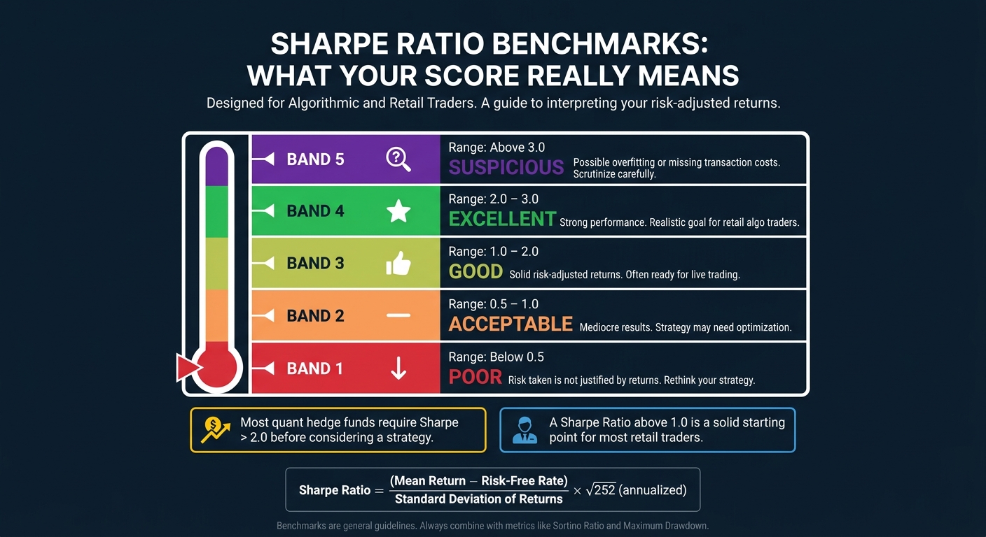
Sharpe Ratio Benchmarks: What Your Score Really Means
Understanding the Sharpe Ratio is essential for evaluating the performance of your trading strategy.
Sharpe Ratio Benchmarks
The Sharpe Ratio becomes more meaningful when compared against benchmarks. Here's a general breakdown of what the numbers indicate:
| Sharpe Ratio Range | Interpretation | What It Means for You |
|---|---|---|
| Below 0.5 | Poor | The risk you're taking isn't justified by the returns. |
| 0.5 – 1.0 | Acceptable | The results are mediocre - your strategy might need tweaking. |
| 1.0 – 2.0 | Good | Shows solid risk-adjusted returns and is often ready for live trading. |
| 2.0 – 3.0 | Excellent | Indicates strong performance and is a realistic goal for many retail algo traders. |
| Above 3.0 | Suspicious | Could signal overfitting or overlooked transaction costs. |
"Most Quantitative hedge funds ignore strategies with an annualised Sharpe ratio of less than 2." - QuantInsti
For most traders, a Sharpe Ratio above 1.0 is a solid starting point, while exceeding 2.0 signals strong performance. However, if your backtests show a Sharpe Ratio higher than 3.0, it’s worth scrutinizing the strategy for potential overfitting or missing costs rather than celebrating it outright.
While these benchmarks provide a useful framework, it’s important to remember that the Sharpe Ratio has its own set of limitations.
Limitations of the Sharpe Ratio in Simulated Trading
Despite its usefulness, the Sharpe Ratio has some notable shortcomings. One of the main issues lies in how it treats volatility. The formula doesn’t differentiate between volatility caused by large gains and that caused by losses. As a result, a strategy with occasional big wins might appear less favorable than a steady, low-return approach.
Another limitation is the assumption that returns follow a normal distribution. In reality, markets are prone to extreme events - like crashes or sudden price spikes - that occur more frequently than a bell curve would suggest. A strategy that seems stable under normal conditions could fail dramatically during these rare but impactful events.
Simulated strategies can also inflate Sharpe Ratios if they exclude realistic costs or rely on short performance histories. For example:
"Calculating Sharpe ratios using daily vs monthly returns can give results 20% different for the same asset. If returns have autocorrelation, the difference can reach 65%." - CAIA Association
To get a more comprehensive view of your strategy’s performance, it’s wise to use additional metrics like the Sortino Ratio or Maximum Drawdown. These metrics can help assess not only efficiency but also how well your strategy handles tough market conditions.
How For Traders Supports Your Simulated Trading

Put your Sharpe Ratio knowledge into action with For Traders. The platform provides tools and challenges designed to help you integrate risk-adjusted performance analysis directly into your trading process.
Using For Traders' Simulated Challenges
For Traders offers Simulated Challenges featuring virtual capital ranging from $6,000 to $100,000. These challenges come with a Trader Dashboard, which allows you to export historical data and track your performance under conditions that mimic real-world trading. Tools like the Lot Size and Earnings Calculators help you fine-tune your risk-return parameters. By maintaining a detailed trade log through the dashboard, you can calculate a more reliable Sharpe Ratio to evaluate your strategies.
"The Sharpe Ratio is one of the most commonly used indicators on the foreign exchange (Forex) market, which can be used to determine the effectiveness of both an individual trading strategy and an investment portfolio." - ForTraders.org
Learning Resources to Improve Your Performance
Apart from challenges, For Traders provides a wealth of educational tools to sharpen your strategies. The For Traders Academy includes video courses, livestreams, and interviews focused on practical trading techniques. For those aiming to improve their Sharpe Ratio, the platform’s blog features guides like "5 Steps to Optimize Sharpe Ratio," packed with actionable advice for enhancing your risk-adjusted returns.
Additionally, the High Performance Coaching program addresses trading psychology, helping you develop the discipline required to manage return volatility and maintain a strong Sharpe Ratio. For even more support, join the For Traders Discord community, where you can discuss strategies and get real-time feedback on your performance.
Conclusion
To compute the Sharpe Ratio for simulated trades, start by deriving periodic returns, subtract the risk-free rate, and then divide by the standard deviation of those returns. Finally, annualize the result using the square root of the number of periods (e.g., √252 for daily data). This process converts raw performance into a practical measure of how effectively your strategy balances returns against the risks it takes. As a general rule, ratios above 1.0 are considered reasonable, while those exceeding 2.0 indicate strong performance. However, relying solely on the Sharpe Ratio can be limiting - combining it with metrics like Maximum Drawdown or the Sortino Ratio offers a broader view of your strategy's resilience.
These calculations not only help you evaluate performance but also provide insights for refining your trading strategies. Simulated trading environments are perfect for testing and improving your approach without incurring financial risk. Platforms like For Traders support this process with features such as structured challenges, a Trader Dashboard to monitor performance, and resources from the For Traders Academy to help you optimize and scale your strategies effectively.
FAQs
Should I use simple returns or log returns?
Log returns are often the preferred choice for calculating the Sharpe Ratio, especially in backtests and performance evaluations. They excel at capturing proportional changes, aggregate seamlessly over time, and deliver consistent measurements of both return and volatility. While simple returns may occasionally be used, most professional research leans toward log returns due to their stability and mathematical advantages. This makes them a more precise tool for analyzing risk-adjusted performance.
How do I adjust the risk-free rate for daily data?
When working with daily data to calculate the Sharpe Ratio, it's important to adjust the risk-free rate to match the daily time frame. To do this, convert the annual risk-free rate into its daily equivalent. Here's how:
- First, divide the annual risk-free rate by 12 to get the monthly rate.
- Then, divide that monthly rate by the typical number of trading days in a month (around 21).
Alternatively, if you're annualizing the Sharpe Ratio, multiply it by the square root of 252, as there are roughly 252 trading days in a year. This ensures consistency between your data and the risk-free rate.
Why can a very high Sharpe Ratio be misleading?
A very high Sharpe Ratio can sometimes give a skewed picture of a strategy's performance. This could happen due to factors like a small sample size, low volatility, or even data mining. These issues might not accurately represent the true risk-adjusted returns, leading to a potentially misleading sense of how effective the strategy really is.
Related Blog Posts
Start Trading with For Traders
Join our platform to test your trading skills, trade virtual capital, and earn real profits. Access educational resources, advanced tools, and a supportive community to enhance your trading journey.
Start your Trading Challenge